Abstract:

We have proposed a method of sensor planning for mobile robot localization using Bayesian network [1]. In this system mobile robot adaptively gathers information to construct a cause-effect-relation in a Bayesian network, and reconstructs the network for sensor planning based on an integrated utility function, then efficient sensing behavior for localization is obtained using inference of the reconstructed network. Experiments in a real environment have been conducted.

sensor planning, mobile robot, localization, Bayesian network, reconstruct

Sensor Planning for Mobile Robot Localization Using Bayesian Network
- Experiments in a real environment -

*Hongjun Zhou (Chuo University), Shigeyuki Sakane (Chuo University)

Introduction

In a complex environment, how to localize mobile robot on its way and navigate it towards a goal is a very fascinating problem to many researchers. Until now, making a global map by sensor information is a mainstream in mobile robot's navigation. A mobile robot localizes itself based on matching local or global sensor information to the map, decides its behavior subsequently by the matching results. However, in the real world, since a lot of uncertainty factors disturb the navigation, it is difficult to use the map-based methods. In this paper we propose adaptive reconstruction of Bayesian network to localize mobile robot.

Tani[5] avoids error of global measurement focus local information only and maps it to motor command space directly. However, this method have no skill recognizing and distinguishing two sets of patterns that hold same sensor information. Asoh et al.[3] developed a mobile robot which navigates based on a prior-designed Bayesian Network, But they have not implemented a sensor planning mechanism. Thrun[2] localizes a mobile robot using Bayesian analysis of probabilistic belief. But this method has not implemented a Bayesian network. Rimey et al.[4] use Bayes nets to recognize table setting, and plan the camera's gaze control based on the maximum expected utility decision rules. However the structure of the Bayes net was fixed.

Prototype system

We use a mobile robot(B14,Real World Interface)(Figure 3) for our research. The mobile robot is driven basically by potential method. On a road with no crossings, the mobile robot searches the maximum value of every glance of sonar scanner, and track the angular direction of the largest sonar value. When it comes to a crossing, robot's action is determined by low level action control. We employ a three-layered Back Propagation Neural Network(BPNN) to map the 8-direction sonar data of the front of mobile robot into action commands at crossings.

Reconstruction algorithm

By taking into account the balance between belief and the sensing cost, we defined an integrated utility function (Eq. 1) and a reconstruction algorithm of the Bayesian network for sensor planning.

$${\bf IU_i = t \times \Delta Bel_i + (1-t) \times (1 - \frac {Cost_{i}}{\sum_{i}Cost_{i}})}$$ (1)

${\bf IU_i}$ denotes the integrated utility (IU) value of sensing node i, ${\bf Cost_{i}}$ denotes the sensing cost of sensing node i, ${\bf Bel_i}$ denotes the Bayesian network's belief while the mobile robot just obtains the evidence of active sensing i only, and ${\bf\Delta Bel_i}$ represents certainty of the belief of sensing node i which contributes to the Bayesian network.

The reconstruction algorithm has two steps [6], STEP (1) completes the refining process of each local network. In other words, Bayesian network will be reconstructed from every local network (active sensing nodes of every crossing) using IU function. STEP (2) combines local networks to the global Bayesian network.

Experiments

To validate the concepts of our system, we perform some experiments using the mobile robot and it's simulator.

Simulation experiments

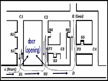
We build an environment to describe the problem as shown in Figure 1. The mobile robot initially navigates by LLAC, and gathers information to make CTPs of the sensing nodes and an original Bayesian network (Figure 2 (a)) In Fig. 1, there are two hidden crossings ( ${\bf F_2, F_3}$) after passing crossings ${\bf B_2}$ and D, respectively. We assume some hidden states (${\bf H_2}$ and ${\bf H_3}$) exist in the Bayesian network. ${\bf H_2}$ (or ${\bf H_3}$) denotes the sensing node sets of the hidden crossings ${\bf F_2}$ (or ${\bf F_3}$), we represent the causal relation between sensing nodes and hidden state as shown in Fig. 2 (a) ( ${\bf C_3}$ and ${\it S_3}$'s parent is ${\bf H_2}$; ${\bf C_4}$ and ${\it S_5}$'s parent is ${\bf H_3}$). The sensed evidence will be propagated from terminal nodes to hidden state node (${\bf H_2}$ or ${\bf H_3}$)), then ${\bf D}$'s belief will be updated by propagation of hidden node's probability. When the ${\it t}$ value (Fig. 2 (c)) of IU function is $0.35$, the original Bayesian network (Fig. 2 (a)) is reconstructed as Fig. 2 (b). Fig. 1 (down) shows the planned path for localization of the mobile robot.

Figure 1: (left) The mobile robot navigates itself by LLAC and some tutorial commands to search the goal (E) and gathers the sensor information actively, then compares the difference of every crossing to construct the CPTs of every sensing node and original Bayesian network. (right) The mobile robot is navigated following the solid line trajectory using inference of reconstructed Bayesian network ${\it (t=0.35)}$.

Figure 2: Reconstruction of the Bayesian network which has hidden states.

Real robot experiments

To validate our algorithm in real environment, we build an experimental environment (Figure 4), and the mobile robot is driven based on a wall-following algorighm. A CCD camera is mounded on the robot to recognize the local environment (color landmark). In the same way as the previous simulation experiments, while the mobile can't localize itself only by local sensing information, the active sensing is performed using sonar sensor (looking for some hollows on the walls). The mobile robot can observe the local sensor information (landmark) by vision to decide whether the position is goal. Firstly the mobile robot performs the active sensing using sonar sensor while it senses the position C isn't goal (Fig.4(left)), and constructs the CPTs of every sensing node. Consequently, the robot balances the localization belief and sensing cost to reconstruct the Bayesian network, then plans it's active sensing action to gather the sensing information and infer the localization of itself based on the reconstructed Bayesian network (Fig.4(right)).

Figure 3: (left) We build a real environment like simulation. (right) We use B14 mobile robot which mounted a camera to observe the local sensing information. The robot actively gathers sensing information via sonar sensor. Since the local environment(opened doors) is identical, the uncertainty of localization is occured, and the mobile robot turns right controled by LLAC to attempt to look for the goal.

Figure 4: (left) The mobile robot turns back and gathers the active information for Bayesian network construction, while it senses the position C isn't goal based on vision; (right) Sensor planning for the mobile robot localization with reconstructed Bayesian network. The robot turns back at the midway of the corridor and havn't necessary to arrive the bottom.

Conclusion and future work

In this paper we conduct some real robot experiments to validate our concept based on an integrated utility function [6]. The system balances the sensing cost and localization belief, and reconstructs the Bayesian network via this function. The mobile robot plans the sensor action using this reconstructed Bayesian network to localize itself. The results of experiments demonstrate the IU function and our reconstruction algorithm effectively cope with the some real environments and complex hierarchical Bayesian network. In the future, we will attempt to learn the structure of Bayesian network from CPTs, and validate our concept using other application.

Bibliography

1

T.Dean et al.,Artificial Intelligence, The Benjamin/Cummings, 1995.

2

S.Thrun, ``Bayesian landmark learning for mobile robot localization'', Machine Learning 33, 41-76, 1998.

3

H.Asoh, Y.Motomura, I.Hara, S.Akaho, S.Hayamizu, and T.Matsui, ``Combining probabilistic map and dialog for robust life-long office navigation'', IROS'96, pp.880-885, 1997.

4

R.D.Rimey and C.M.Brown,'' Where to look next using a Bayes nets, Incorporating geometric relations'', Proc. European Conference on Computer Vision, 1992.

5

J.Tani,''Model-based learning for mobile robot navigation from the dynamic Systems Perspective'',IEEE Trans.on SMC, Part B (Special Issue on Robot Learning),Vol.10,No.1,pp153-159.1977.

6

H.J.Zhou S.Sakane, ``Sensor Planning for Mobile Robot Localization Using Bayesian Network Inference'', ISATP'2001, pp.7-12, 2001.

7

H.J.Zhou S.Sakane, ``Sensor Planning for Mobile Robot Localization -An approach using Baysian network inference-'', RSJ'2000, Vol.3, pp.991-992,2000.

About this document ...

Sensor Planning for Mobile Robot Localization Using Bayesian Network
- Experiments in a real environment -

This document was generated using the LaTeX2HTML translator Version 99.2beta8 (1.46)

Copyright © 1993, 1994, 1995, 1996, Nikos Drakos, Computer Based Learning Unit, University of Leeds.
Copyright © 1997, 1998, 1999, Ross Moore, Mathematics Department, Macquarie University, Sydney.

The command line arguments were:
latex2html -local_icons -split 0 rsj2001.tex

The translation was initiated by on 2001-10-09